Explaining Node-based workflow for AI image generation

Before we begin

I will be using ComfyUI as basis for pictures but the same concepts apply to Invoke AI and a1111 UIs. This is basically how they handle stuff under the hood.

Also, do keep in mind that I’m not an expert on the subject by any means. I just happen to have spent a while scavenging the web for documentation and overall trying to understand how AI-image-generation works. My field of work is computer graphics and game engines. A bit distant from Machine Learning.

If you have suggestions/feedback or want to correct me on something, feel free to reach out to me.

So, what exactly are nodes?

If you’re coming from one of the usual UIs for AI image generation, you might be wondering what the heck are nodes and why are they so interesting for some peoples.
The truth is that, unless you want to delve deeper into how an image gets generated or you need more control over the entire process, you don’t need to know anything about nodes.

But if you are interested in learning more about how AI image generation works, or you want to have more control over the entire process, then by all means, keep on reading…

In short

• Nodes are just a clear representation of the flow of data when generating an image using AI.
• The advantage of using nodes it that you can thoroughly customize the entire image generation process by yourself. You have sampler nodes, conditioning nodes, input nodes, output nodes…
• Without going into explaining one by one all possible nodes and combinations (good luck, this would be a gigantic wall of text, more than it is already), I can give you a basic overview of how the basic stuff we do in a1111/invoke ai work under the hood.

Checkpoints:

Or: what models are actually involved in generating an image

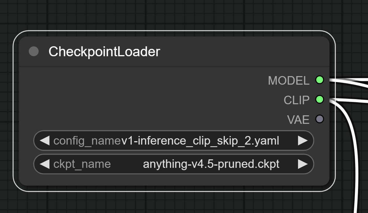
Also known as models, they need to be loaded and unpacked to memory to be used. Each checkpoint can optionally also contain an integrated CLIP and VAE model baked into itself.

CLIP Model

A CLIP model is a Text Encoder, in layman terms its the black box that accepts your input and translates it to the model itself, so that it can generate an image containing what you want to see.

The actual checkpoint

The model itself takes a starting point (in case of txt2img, a randomized noise image; in case of img2img a “blurred”, more noisy version of your starting image), and starts denoising. By progressively removing noise from the current image in a way that statistically represents an image that resembles more your positive input (positive conditioning) and less your negative input (negative conditioning), it slowly converges to an image in “latent space”.

VAE Model

A VAE model then clears the latent space and returns you an image. You can think of this like the final step of developing an photograph in the old days, the last bath to permanently fix the colors before pulling it out and letting it dry.

Latent Space

A very quick introduction to what the AI really sees

Latent Space is a term that will come out multiple times during this read, so let’s take a moment to explain what it really is.

In terms of a Stable-Diffusion model, you can think of this as a canvas that the model uses to draw the image onto. But it’s only a bunch of numbers really, and it’s up to the model and the sampler to interpret them accordingly.

Additionally, this “image” is not a single layer, but muliple of them. And by applying conditioning over the current latent space, step after step, the decoded image that is generated from it, is going to be more and more similar to the conditioning you set at the beginning.

When you start generating an image from a text prompt only, you initialize the latent space with a bunch of random values. The random values are chosen thanks to a seed, allowing repeatability.

When generating from an image the latentspace is initialized with data from your image after the VAE model has encoded it into latent space.

Conditioning:

What you think you’re saying is not necessarly what CLIP is understanding

Let’s spend a moment to talk about conditioning and how CLIP actually sees your input.

CLIP is a neural network that has been trained to understand the meaning of images and text. It’s a black box that takes your input and translates it to a vector of numbers that represents the meaning of your input.

The words you input are going to be split into tokens, and each token is going to be translated to a vector of numbers. (Think of it like a set of numbers that correspond to that token). The same happens with the images you input. The vectors are then compared with the current latent image while is being generated and the result is a number that represents how much the image and the text are similar. The higher the number, the more similar they are.

Tokens

The vocabulary of the model

But what exactly is a token? A token is generally a set of characters that the CLIP model has associated a meaning to. The most basic token you always use while writing a conditioning is the , comma. The CLIP model has been trained to understand that a comma is a separator between words and that it should be basically ignored when analyzing the meaning of the input.

Note: commas do still have an effect on the conditioning, they in fact split a conditioning prompt into sections, this is expecially true for models that are trained over more verbose inputs. This is why you can use commas to separate different sections of your conditioning, like “a cat, a dog, a bird” and the model will hopefully generate an image that contains all three animals.

“Clip Styles”

A “dialect” for models

In-between quotes because I don’t really know what’s the correct lingo here.

But, as every model ships with its CLIP model inside, some models require a different style of conditioning. For example, a lot of the anime models are trained to react to danbooru tags used as conditioning. Describing a scene in natural language (as you would to a normal person) will still work but will not be as effective. Stable Diffusion model and a bunch of the photorealistic/artistic models instead will not be really effective on danbooru tags, but will work better with natural language.
This always depends on the model you’re using, and the best way to find out is to either read the readme left by the author, looking into the readmes for the models that the specific model derives from or just by experimenting.

Negative Conditioning:

What you don’t want to see. More or less…

This is conditioning but in the opposite (negative) way. You can use it to tell the model what you don’t want to see in the image.

Everything I said about conditioning applies to negative conditioning as well. Only that with negative conditioning the model will try to have the derived vectors from the tokens to be as distant as possible from the current latent image.

Negative conditioning Myths

Let’s try to dispel some myths about negative conditioning:

• bad hands doesn’t works as well as you think. bad is a token and hands is another. The model doesn’t have a clue about what bad hands are on their own. using (hands) will result in more or less the same result, with 1 less token.
• Longer conditioning prompts are not always better. If you exceed 75 tokens in your positive or negative token, the generation speed will almost halve itself because of the extra required processing (the model can only work with 75 tokens at the time, so it has to split the conditioning in chunks of 75 tokens and process them one by one). This is why you should try to keep your conditioning as short as possible.
• A good way to fix this without exceeding the 75 tokens count is to use embeddings.

Embeddings:

Condensing informations into a single token

Also called “Textual Inversion Embeddings”.

Embeddings are a way to condense a part of your conditioning into a single token. They are not a collection of tokens per se, rather a definition of where your concept is placed in the latent space.

Under the hood

Imagine again the latent space, there are a bunch of zones (or layers) that define specific features, like the eyes, the nose, the mouth, the hair, the clothes, the background, etc.
Embeddings are a way to tell the model “I want to see this in the image, and I want it to be as close as possible to these values”. It does this by offsetting specific groups of values in the latent space.

Embeddings in practice

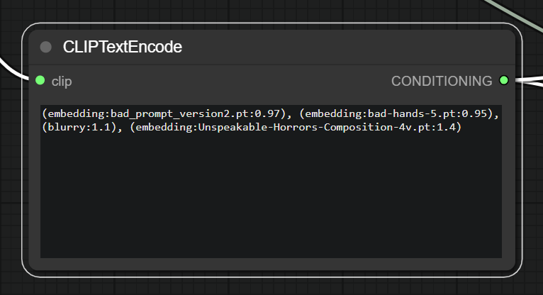
The result is a quick way to only consume a single token and still have the same effect of a lot of tokens used as conditioning. They are now really popular in negative prompts to strongly condition the model away from bad hands, bad anatomy, bad composition and so on…

They can, of course, also be used as positive conditioning, but that job is often left to LoRAs nowadays.

LoRAs

Low-Rank Adaptations

Fast and small

LoRAs are a recetly introduced technique for fine-tuning a model on the fly, without the need of having hundred of images and without needing long train times and huge file sizes, compared to DreamBooth models.

How do they work?

A model is basically a gigantic matrix of numbers. Fine tuning changes some of those numbers in the matrix to make the model better at generating images that are similar to the ones you used for fine tuning. By saving only the difference between the original model and the model after the fine tuning, a LoRA will be both small and fast to be applied. Also, you can easily apply multiple of them at the same time and they can work across multiple models (with some caveats, for example: a LoRA trained over anime Images will often not play nice with a model that tries to output photorealistic images).

Actually how do they work under the hood?

Nah. This is currently the easiest to understand explanation I can give you. I have a decent idea of how they work under the hood, but I do not think I can explain it in a way that is both easy to understand and accurate. So I’ll not go into details for now.

LoRAs in practice

When you apply a lora, you basically apply the fitting over the model currently loaded in memory. Some LoRAs will work best if the positive/negative conditioning contain certain tokens. Others will work fine as long as they are loaded. Some will be really strong, other will be much more lenient. It all depends on how the LoRA was trained. As ususal, the best way to find out is to experiment and to read the readme left by the author (if present).

Pipelines

How basic workflows actually work

So far we adressed the basic building blocks that we use in any UI for interacting with the model. Let’s now take a look at how some of the basic things we usually do actually work under the hood.

Plain txt2img pipeline

Everyone should be familiar with this, it’s by far the most basic way to actually obtain an image. In fact, this is the bare minimum setup you need to get an image from the model.

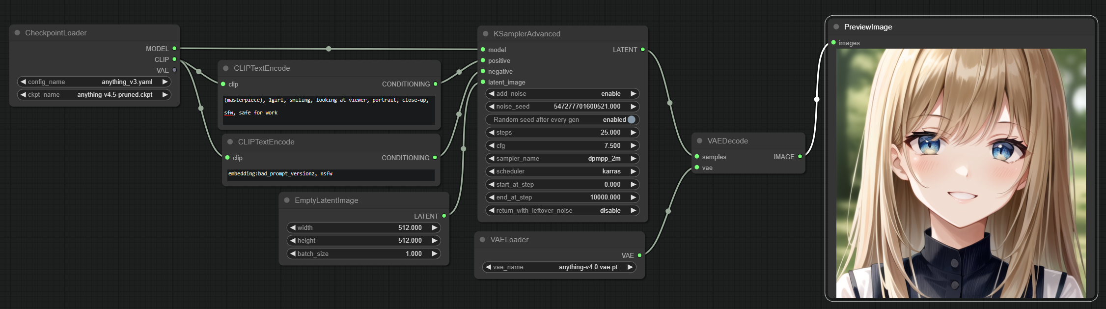
Let’s look at it step by step, or rather, node by node:

1. The CheckpointLoader node loads the model and the associated CLIP model and if available a VAE model too.
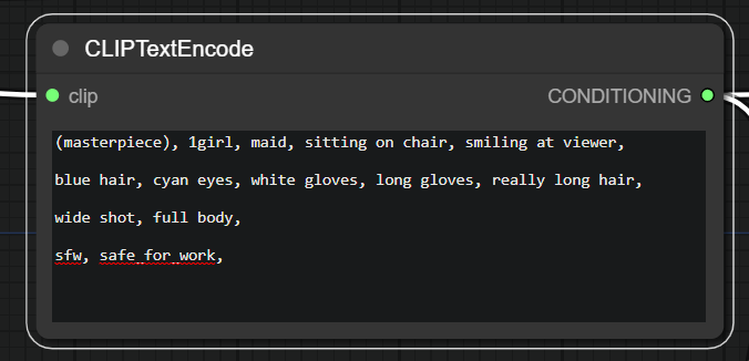
2. Two CLIPTextEncode nodes are used, one for supplying the positive conditioning and one for the negative conditioning. They both use the CLIP model loaded in the previous step and output a conditioning.
3. An empty latent image is created at the specified resolution.
4. Both conditionings are supplied alongside the model and the empty latent image to the sampler, which actually adds noise to the latter, then starts the generation process.
5. A VAE gets loaded because we didn’t have one before.
6. the VAEDecode node takes the latent samples from the sampler and uses the VAE model to decode the latent samples into an image.
7. Said image gets finally displayed as a preview (optionally also saved to the disk.)

Adding LoRAs to the mix

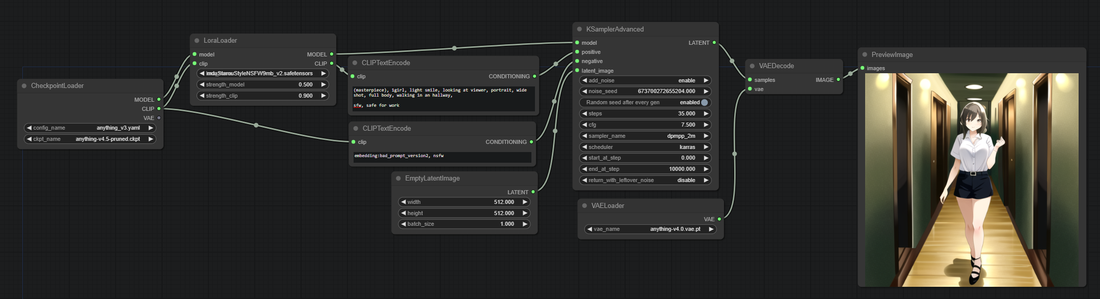
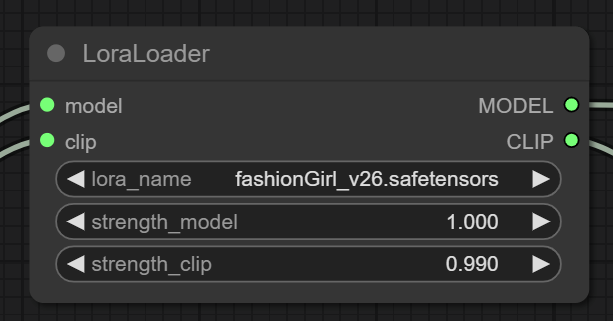
Adding LoRAs to the mix is pretty simple. We add a LoRA node between the CheckpointLoader and the CLIPTextEncode nodes. The LoRA node will load the LoRA and apply it to the CLIP model before the CLIPTextEncode nodes are used. Additionally it will also apply the LoRA to the actual model.

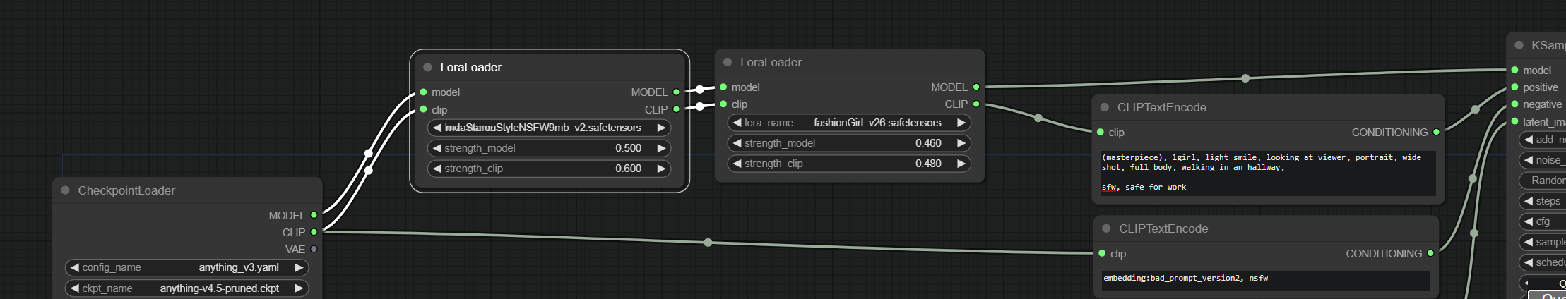
Multiple LoRAs? just chain multiple nodes together.

HiresFix

If you’ve been generating images for a while, you probably heard someone mention “HiResFix”. It’s a technique that allows you to generate images at a higher resolution than the one the model was trained on. Most models are trained at 512x512 images, some at 768x768 but what if you want to go higher? Well, something like this might happen:

You can clearly see how there are actually 2 images there, and the model doesn’t really know how to blend this all together. This is where HiResFix comes in.

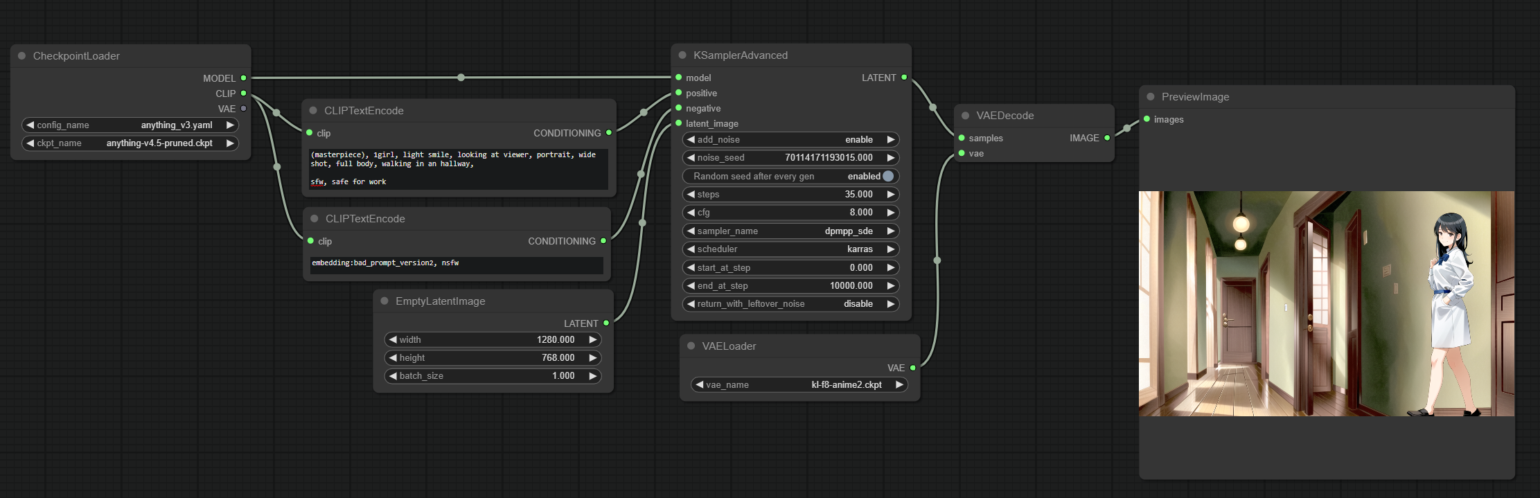
Here’s how HiResFix looks like in a node based editor:

Okay, this might look overwhelming at first, but it’s actually pretty simple. Let’s break it down:

• The txt2img block (in blue) is the same as the one we saw before. The only difference is that we are using a 640x384 empty latent image instead of a 512x512 one. This is because we will then upscale that to a factor of 2 to get a 1280x768 image at the end.

• The yellow block is totally optional, thats just me fetching what the image looked like before going trough the HiResFix process.

• The green block is where the magic happens.

  • The latent image resulting from the txt2img process is now sent trough a LatentUpscale node.
  • This node is going to upscale the latent image by a factor of 2. This means that the 640x384 latent image will become a 1280x768 latent image.
  • We then feed this image to the sampler, which will add noise (notice the denoise parameter) and iterate over it. But because now it has a starting point, and the denoise value is not too high, it will just upscale the image and add detail instead of getting confused and spitting out two images one next to eachother.

• We then decode the image as usual and we get a nice 1280x768 image.

Notice that some details changed. This is depending on the denoise value. You can thing of this as how much from 0 to 1 we are going to blur the image. If you set it to 0, the image will be exactly the same as the one we started with. If you set it to 1, the image will be completely blurred and we will end up with a completely new image. The sweet spot is somewhere in the middle, but it depends on the model and the image you are generating. Usually around 0.55-0.65 is where it works best.

And that’s it for how HiResFix works. It’s not complicated, but it can feel overwhelming just by looking at it in a node based enviroment.

And this goes to show that even though the node based enviroment is very powerful, it’s not always the best way to work with this kind of stuff.

The real downside of node based editors

As soon as complexity kicks in, it becomes a rats nest. It can quickly become a nightmare to work with nodes and you can end up with a lot of headaches when trying to understand why something doesn’t work.

But its a good way to play around with stuff and understand how it works internally. Also, if you ever decide to work with it by using scripting, it will be really easy to reconstruct your pipelines there.

And if you don’t know how to program, I guess is a good way to prototype a good pipeline or achieve results otherwise impossible with the standard UIs.

Conclusion

This became a really long article. I hope you learned something from it. This has also been a good excuse for myself to go slightly deeper into how some stuff works internally. I’d love to expand on this in the future, maybe with another article about more advanced techniques on node based image generation, upscaling techniques maybe? Img2img? Detail enhancement? But for now I think this is enough.

Till next time… have fun generating images!